Example of WDf usage with multi data segments and multi-processing¶

author: Elena Cuoco

Cuoco et al., Wavelet-Based Classification of Transient Signals for Gravitational Wave Detectors DO - 10.23919/EUSIPCO.2018.8553393

Please note that many packages, as graphic one or logging are not part of WDF docker, but you can install them locally or use your preferred ones

[1]:

# import libraries
import time
import os
from pytsa.tsa import *
from pytsa.tsa import SeqView_double_t as SV
from wdf.config.Parameters import *
from wdf.processes.wdfUnitDSWorker import *
from wdf.processes.wdfUnitWorker import *
import logging
import coloredlogs
#select level of logging
coloredlogs.install(isatty=True)

logging.basicConfig(level=logging.DEBUG)

[2]:

new_json_config_file = True    # set to True if you want to create new Configuration

if new_json_config_file==True:
    configuration = {
  "window":1024,
  "overlap":768,
  "threshold": 0.2,
  "file": "./data/test.gwf",
  "channel": "H1:GWOSC-4KHZ_R1_STRAIN",
  "run":"offLine",
  "len":10.0,
  "gps":1167559608,
  "segments":[[1167559008,1167559408],[1167559408,1167560008],[1167560008,1167560308]],
  #"segments":[[1167559608,1167560008] ],
  "outdir": "local_dir/",
  "dir":"local_dir/",
  "ID":"WDF_test",
  "ARorder": 1000,
  "learn": 200,
  "preWhite":2,
  "ResamplingFactor":2,
  "LowFrequencyCut":12,
  "FilterOrder":6,
  "nproc":4
}

    filejson = os.path.join(os.getcwd(),"inputWDF.json")
    file_json = open(filejson, "w+")
    json.dump(configuration, file_json)
    file_json.close()

logging.info("read parameters from JSON file")
par = Parameters()

filejson = "inputWDF.json"
try:
    par.load(filejson)
except IOError:
    logging.error("Cannot find resource file " + filejson)
    quit()

par.print()

2023-03-29 14:18:51 hal2022 root[4076457] INFO read parameters from JSON file

{   'ARorder': 1000,
    'FilterOrder': 6,
    'ID': 'WDF_test',
    'LowFrequencyCut': 12,
    'ResamplingFactor': 2,
    'channel': 'H1:GWOSC-4KHZ_R1_STRAIN',
    'dir': 'local_dir/',
    'file': './data/test.gwf',
    'gps': 1167559608,
    'learn': 200,
    'len': 10.0,
    'nproc': 4,
    'outdir': 'local_dir/',
    'overlap': 768,
    'preWhite': 2,
    'run': 'offLine',
    'segments': [   [1167559008, 1167559408],
                    [1167559408, 1167560008],
                    [1167560008, 1167560308]],
    'threshold': 0.2,
    'window': 1024}

It is important that you define correctly the parameters in the configuration files. WDf is a pipeline which performs a series of steps before producing triggers for transient signals in your data. Here it is the list of parameters you can fix in your configuration file.

ARorder = order of AutoRegressive model for whitening
ID = identification numer for your run
ResamplingFactor = the ratio between the original sampling frequency and the downsampled one
channel = the name of the channel in you .gwf o .ffl file you want to analyze
dir = where to find the parameters
file = file to be anlyzed
gps = the starting time for for analysis (overwritten by values in segments)
learn = the length in seconds of the data you will use to estimate AR parameters
len = the time window in second of data loaded in you loop
nproc = the number of processors you will use
outdir = where you want to save the results
overlap = overlapping number between 2 consecutives windows for WDF analysis
prewhite = the number of iter to pre-heat the whitening procedure (leave as it is)
run = additional tag for your data run
segments = 1 or more segments defined as [start time, end time] where you will run WDF, usually 1 segment/processor
threshold = the minimum value for WDF snr to identify a trigger
window = the analyzing window in point for WDF. It should be a power of 2

If you set the par.dir or par.outdir as relative path, we need to give the absolute path.

[3]:

import os
par.dir=os.getcwd()+'/'+par.dir
par.outdir=os.getcwd()+'/'+par.outdir

Load information for sampling frequency¶

[4]:

strInfo = FrameIChannel(par.file, par.channel, 1.0, par.gps)
Info = SV()
strInfo.GetData(Info)
par.sampling = int(1.0 / Info.GetSampling())
if par.ResamplingFactor!=None:
    par.resampling = int(par.sampling / par.ResamplingFactor)
    logging.info("sampling frequency= %s, resampled frequency= %s" %(par.sampling, par.resampling))
del Info, strInfo

2023-03-29 14:18:52 hal2022 root[4076457] INFO sampling frequency= 4096, resampled frequency= 2048

Launch WDF runs¶

The fullPrint option is important to save information about the WDF triggers¶

fullPrint = 0 –> you save only the metaparameters for the triggers
fullPrint = 1 –> you save the metaparameters and the wavelet coefficients for that trigger
fullPrint = 2 –> you save the metaparameters and the reconstructed waveform for that trigger
fullPring = 3 –> you save the metaparameters, the wavelet coefficients and the reconstructed waveform for that trigger in the ‘window’ time (window/sampling frequency)

[5]:

import multiprocessing as mp
print("Number of processors: ", mp.cpu_count())
pool = mp.Pool(par.nproc)

wdf=wdfUnitDSWorker(par,fullPrint=2)
pool.map(wdf.segmentProcess, [segment for segment in par.segments])
pool.close()

Number of processors:  32

2023-03-29 14:18:52 hal2022 root[4076576] INFO Analyzing segment: 1167560008-1167560308 for channel H1:GWOSC-4KHZ_R1_STRAIN downsampled at 2048Hz
2023-03-29 14:18:52 hal2022 root[4076575] INFO Analyzing segment: 1167559408-1167560008 for channel H1:GWOSC-4KHZ_R1_STRAIN downsampled at 2048Hz
2023-03-29 14:18:52 hal2022 root[4076574] INFO Analyzing segment: 1167559008-1167559408 for channel H1:GWOSC-4KHZ_R1_STRAIN downsampled at 2048Hz
2023-03-29 14:18:52 hal2022 root[4076575] INFO Start AR parameter estimation
2023-03-29 14:18:52 hal2022 root[4076574] INFO Start AR parameter estimation
2023-03-29 14:18:52 hal2022 root[4076576] INFO Start AR parameter estimation
2023-03-29 14:19:27 hal2022 root[4076575] INFO Estimated sigma= 4.0675451444151897e-22
2023-03-29 14:19:27 hal2022 root[4076576] INFO Estimated sigma= 4.0062637269449494e-22
2023-03-29 14:19:27 hal2022 root[4076574] INFO Estimated sigma= 4.0023147527036696e-22
2023-03-29 14:19:32 hal2022 root[4076575] INFO Starting detection loop
2023-03-29 14:19:32 hal2022 root[4076576] INFO Starting detection loop
2023-03-29 14:19:32 hal2022 root[4076574] INFO Starting detection loop
2023-03-29 14:22:25 hal2022 root[4076576] INFO analyzed 300 seconds in 212.9326889514923 seconds
2023-03-29 14:23:22 hal2022 root[4076574] INFO analyzed 400 seconds in 270.102082490921 seconds
2023-03-29 14:25:12 hal2022 root[4076575] INFO analyzed 600 seconds in 379.5118489265442 seconds

In the output dir with ‘run’ tag you will find the estimated AR coefficients, and a .csv files containing the trigger lists

Let’s have a look at the results¶

[6]:

import pandas as pd

import glob

dirName = par.outdir # use your path
all_files = glob.glob(os.path.join(dirName, "*","*.csv"))     # advisable to use os.path.join as this makes concatenation OS independent
df_from_each_file = (pd.read_csv(f) for f in all_files)
triggers  = pd.concat(df_from_each_file, ignore_index=True)

[7]:

triggers.shape

[7]:

(5810, 1035)

[8]:

import matplotlib.pylab as plt
pd.set_option('display.max_rows', 999)
pd.set_option('max_colwidth',100)
pd.set_option('display.float_format', lambda x: '%.3f' % x)
import numpy as np

%matplotlib inline
# Alternatives include bmh, fivethirtyeight, ggplot,
# dark_background, seaborn-deep, etc
plt.style.use('ggplot')
plt.rcParams['font.monospace'] = 'Ubuntu Mono'
plt.rcParams['font.size'] = 10
plt.rcParams['axes.labelsize'] = 10
plt.rcParams['axes.labelweight'] = 'bold'
plt.rcParams['xtick.labelsize'] = 8
plt.rcParams['ytick.labelsize'] = 8
plt.rcParams['legend.fontsize'] = 10
plt.rcParams['figure.titlesize'] = 12
plt.rcParams['figure.figsize'] = (14, 10)

colors = np.array([x for x in 'bgrcmykbgrcmykbgrcmykbgrcmyk'])
colors = np.hstack([colors] * 20)
plt.figure(0)
print (triggers.shape)

triggers.head(10)

(5810, 1035)

[8]:

	gps	gpsPeak	duration	EnWDF	snrMean	snrPeak	freqMin	freqMean	freqMax	freqPeak	...	rw1014	rw1015	rw1016	rw1017	rw1018	rw1019	rw1020	rw1021	rw1022	rw1023
0	1167559009.000	1167559009.421	0.453	0.290	0.256	1.786	62.000	148.346	250.000	136.000	...	0.000	-0.000	-0.000	-0.000	-0.000	-0.000	-0.000	-0.000	-0.000	0.000
1	1167559009.125	1167559009.421	0.500	0.331	0.275	1.809	62.000	155.500	274.000	116.000	...	-0.000	-0.000	-0.000	0.000	0.000	0.000	0.000	0.000	0.000	0.000
2	1167559009.250	1167559009.421	0.473	0.275	0.248	1.734	58.000	153.423	266.000	116.000	...	-0.000	0.000	0.000	0.000	0.000	0.000	0.000	-0.000	-0.000	0.000
3	1167559009.375	1167559009.421	0.477	0.235	0.220	1.628	48.000	154.846	272.000	140.000	...	0.000	0.000	0.000	0.000	0.000	-0.000	-0.000	-0.000	-0.000	-0.000
4	1167559011.375	1167559011.782	0.500	0.305	0.219	1.788	88.000	173.769	282.000	112.000	...	0.000	0.000	0.000	0.000	0.000	-0.000	-0.000	-0.000	-0.000	-0.000
5	1167559011.500	1167559011.782	0.404	0.311	0.224	1.782	86.000	169.269	280.000	124.000	...	-0.000	-0.000	0.000	0.000	0.000	0.000	0.000	0.000	0.000	0.000
6	1167559011.625	1167559011.782	0.500	0.350	0.255	1.769	78.000	170.000	302.000	122.000	...	-0.000	-0.000	-0.000	0.000	0.000	0.000	0.000	0.000	0.000	0.000
7	1167559011.750	1167559011.782	0.473	0.369	0.278	1.794	70.000	168.385	298.000	138.000	...	0.000	0.000	0.000	0.000	0.000	0.000	0.000	0.000	-0.000	-0.000
8	1167559011.875	1167559012.096	0.461	0.252	0.221	1.293	56.000	164.808	318.000	156.000	...	0.000	0.000	0.000	0.000	0.000	-0.000	-0.000	-0.000	-0.000	-0.000
9	1167559012.000	1167559012.096	0.458	0.246	0.219	1.269	54.000	174.000	356.000	156.000	...	-0.000	-0.000	-0.000	-0.000	-0.000	-0.000	-0.000	0.000	0.000	0.000

10 rows × 1035 columns

<Figure size 1400x1000 with 0 Axes>

[9]:

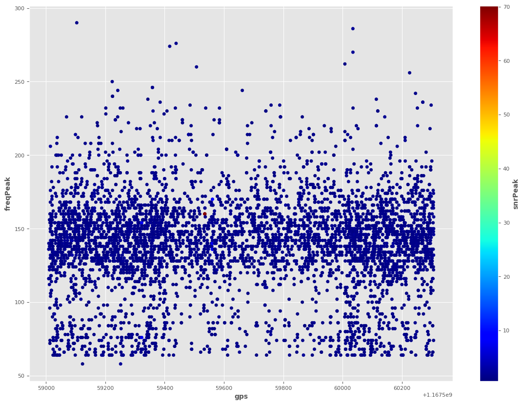
ax2 = triggers.plot.scatter(x='gps',
                      y='freqPeak',
                      c='snrPeak',
                      colormap='jet')

../../_images/structure_examples_Multi-WDF_20_0.png

[10]:

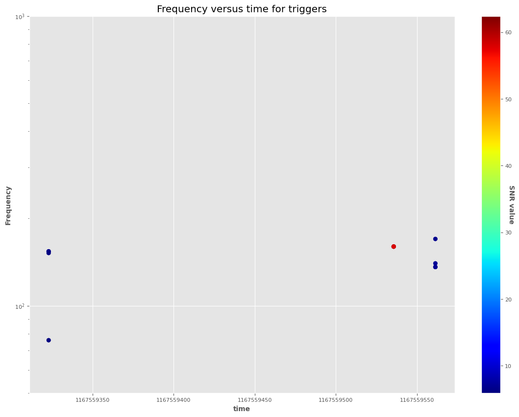
df=triggers[triggers['snrPeak']>4]

[11]:

plt.figure(0)
print (df.shape)

from matplotlib.ticker import FormatStrFormatter

sc = plt.scatter(df.gpsPeak,
                 df.freqPeak,c=df.EnWDF, cmap='jet')

# legend
cbar = plt.colorbar(sc)
cbar.ax.set_yticklabels(['5','10', '20', '30', '40', '50', '60','>60'])
cbar.set_label('SNR value', rotation=270)

plt.ylim(50, 1000)
plt.yscale('log')
plt.gca().get_xaxis().get_major_formatter().set_useOffset(False)
plt.gca().get_xaxis().get_major_formatter().set_scientific(False)
plt.xlabel("time")
plt.ylabel("Frequency")
plt.title("Frequency versus time for triggers")

(12, 1035)

/tmp/ipykernel_4076457/2239143324.py:11: UserWarning: FixedFormatter should only be used together with FixedLocator
  cbar.ax.set_yticklabels(['5','10', '20', '30', '40', '50', '60','>60'])

[11]:

Text(0.5, 1.0, 'Frequency versus time for triggers')

../../_images/structure_examples_Multi-WDF_22_3.png

[12]:

df=triggers.sort_values('EnWDF', ascending=False)

[13]:

df.head(10)

[13]:

	gps	gpsPeak	duration	EnWDF	snrMean	snrPeak	freqMin	freqMean	freqMax	freqPeak	...	rw1014	rw1015	rw1016	rw1017	rw1018	rw1019	rw1020	rw1021	rw1022	rw1023
4255	1167559535.375	1167559535.639	0.019	6.242	4.661	70.169	76.000	152.577	262.000	160.000	...	-0.000	-0.000	-0.000	-0.000	-0.000	-0.000	-0.000	-0.000	-0.000	-0.000
4254	1167559535.250	1167559535.639	0.019	6.219	4.659	70.154	74.000	146.962	260.000	160.000	...	0.000	0.000	0.000	0.000	0.000	0.000	0.000	0.000	0.000	0.000
4256	1167559535.500	1167559535.639	0.019	6.170	4.658	70.118	76.000	150.308	262.000	160.000	...	-0.000	-0.000	-0.000	-0.000	-0.000	0.000	0.000	0.000	0.000	0.000
4257	1167559535.625	1167559535.639	0.019	5.798	4.624	69.640	80.000	152.192	264.000	160.000	...	0.000	0.000	0.000	0.000	0.000	0.000	0.000	-0.000	0.000	0.000
4341	1167559560.875	1167559561.331	0.276	0.706	0.529	8.874	58.000	156.846	276.000	140.000	...	0.000	0.000	0.000	0.000	0.000	0.000	0.000	-0.000	-0.000	-0.000
4343	1167559561.125	1167559561.331	0.107	0.687	0.517	8.830	58.000	152.923	278.000	136.000	...	0.000	0.000	0.000	0.000	0.000	0.000	0.000	0.000	0.000	-0.000
1673	1167559322.500	1167559322.928	0.497	0.685	0.474	7.734	54.000	146.731	240.000	154.000	...	0.000	0.000	0.000	0.000	0.000	-0.000	-0.000	-0.000	0.000	0.000
4344	1167559561.250	1167559561.331	0.018	0.679	0.506	8.830	68.000	149.731	222.000	170.000	...	0.000	0.000	0.000	0.000	0.000	0.000	0.000	-0.000	-0.000	-0.000
4342	1167559561.000	1167559561.331	0.276	0.675	0.522	8.674	58.000	155.308	276.000	136.000	...	0.000	0.000	0.000	0.000	0.000	0.000	-0.000	-0.000	-0.000	-0.000
1674	1167559322.625	1167559322.928	0.411	0.648	0.462	7.642	62.000	150.154	240.000	154.000	...	0.000	0.000	0.000	0.000	0.000	0.000	-0.000	-0.000	-0.000	-0.000

10 rows × 1035 columns

[14]:

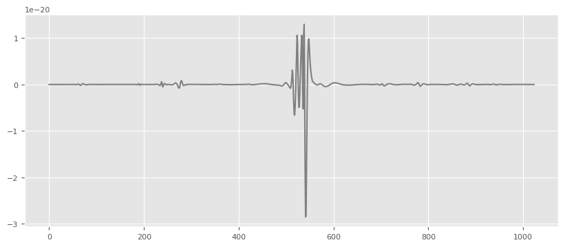
wav=np.array(triggers.loc[triggers['EnWDF'].idxmax()][11:].values)

[15]:

import matplotlib
import matplotlib.pyplot as plt
matplotlib.rcParams['agg.path.chunksize']=10000
%matplotlib inline

plt.figure(figsize=(10,4)),
plt.plot(wav,'gray',label='h'),

[15]:

([<matplotlib.lines.Line2D at 0x7fc742d42310>],)

../../_images/structure_examples_Multi-WDF_26_1.png

[16]:

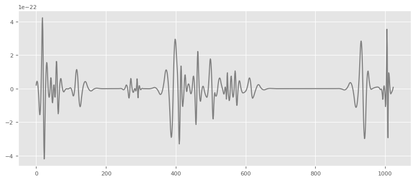
wav=np.array(triggers.loc[11][11:].values)

plt.figure(figsize=(10,4)),
plt.plot(wav,'gray',label='h'),

[16]:

([<matplotlib.lines.Line2D at 0x7fc742d950d0>],)

../../_images/structure_examples_Multi-WDF_27_1.png

[ ]: